Comparison is one of the most common things we do with Excel. Naturally, there are so many ways to compare 2 lists of data using Excel. We have discussed various techniques for comparison earlier too,
- Compare 2 lists using conditional formatting
- Even faster way to compare lists
- Compare lists using row differences
Today, I want to share an interesting comparison problem with you.
Lets say you run a small shop which sells some highly specialized products. Now, since your products require quite some training before customers can buy them, you keep track of all product queries and arrange demos.
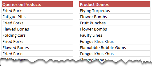
After a hectic week, you are staring at 2 lists. One with product queries, another with product demos.
And you have 2 burning questions,
1. Did we finish all the queries we had?
2. Should I go get some coffee?
Lets answer question number 2. Yes, you can get some coffee. Go, enjoy it now
Back already?!? Good. Now, lets answer the question 1.
Compare 2 Lists Visually using Conditional Formatting
[Note: this article is inspired by Reepal's comment.]
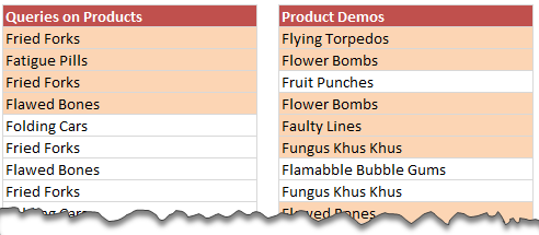
You would like to highlight the lists as shown below, so that you would know whether each product query is fulfilled or not.
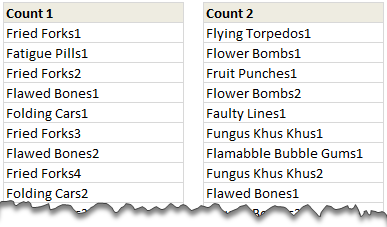
Step 1: Create 2 more lists, with count of products
In order to compare our lists, we need some help. We will create 2 more lists like this:
How do we generate these lists?
Assuming our original data is in B6:B33 and D6:D33,
- In a blank cell (lets say in F6), write =B6&COUNTIF(B$6:B6,B6)
- This gives the count of first product up to that point, ie, Fired Forks1.
- Now drag & fill the formula down until F33
- Do the same in column H, but use the formula =D6&COUNTIF(D$6:D6,D6)
- Fill this until H33
Step 2: Name these new lists
Now that we have created 2 more lists, lets give them names. Select the range F6:F33, go to Formula ribbon and click on “Define Name”. Name the range count1s
Do the same for range H6:H33 and name it count2s
Stpe 3: Apply Conditional Formatting to First List (Product Queries)
Now that we have done all the background work, lets visually compare the data. Select the first list (B6:B33) and go to Conditional Formatting > New Rule
We need to write a rule such that we would highlight all the items in list 1 whenever there is a match in list 2.

The rule is =COUNTIF(count2s,$F6)>0
It means, is the value in F6 present in 2nd list?
in other words, does the first product query has a corresponding product demo?
Set the formatting as you want. Click ok.
Step 4: Apply conditional formatting to Second List
Use the same logic, but this time the rule becomes =COUNTIF(count1s,$H6)
That is all, we have visually compared the two lists.
If you feel like, you can go back for one more cup of coffee.
Download Example Workbook
Click here to download the example workbook – Compare 2 lists visually and play with it. Examine the formulas in columns F & H. Also examine the conditional formatting rules to understand how this works.
How do you compare lists of data?
For me comparison is an everyday task. I rely in several techniques, some quick and dirty, others a bit more elaborate. For quick comparisons, I use either row differences or highlight duplicates rule. For elaborate comparisons, I use COUNTIF, VLOOKUP or other formula based techniques.
What about you? How do you compare lists of values? What techniques and tips you suggest. Please share using comments.
Want to learn Excel Formulas?
If you want to learn Excel formulas so that you can compare, analyze and present better, then please consider joining my Excel Formula Crash Course. This is an 8 hour online training program aimed to make you awesome in Excel formulas. We teach more than 40 every day formulas with loads of real-world examples, practice material & homework.
没有评论:
发表评论