Display Contact Group Member Count

From Code for Excel and Outlook

Display Contact Group Member Count:

Sorry for the lack of posts lately. I've been working on the next version of Random Data Generator, and my home network connection wasn't working for the past few days.

In Display the Total Number of Members in a Contact Group there is a method for displaying the number of members of a contact group (aka distribution list).

There is an easier way, using VBA:

Sub GetDistListCount()

Dim dl As Outlook.DistListItem

Set dl = ActiveExplorer.Selection.item(1)

MsgBox "There are " & dl.MemberCount & " member(s) in this contact group."

End Sub

Just go to your Contacts folder, select a distribution list item and run this code. There is no error handling here, just a simple procedure to display the number of members of the group.

Related Articles:

• June 23, 2011 -- Manage your email overload
• March 7, 2011 -- Get Word Count in VBA
• January 31, 2011 -- Add photos to Contacts in bulk using VBA in Outlook

Display Contact Group Member Count is Copyright © JP Software Technologies. All Rights Reserved.

Finding the 2nd, 3rd, 4th … MATCH()

From Daily Does of Excel

Finding the 2nd, 3rd, 4th … MATCH():

Excel’s MATCH() function will return the relative location of the first occurrence that satisfies the match criterion (the lookup_value) within the specified array (the lookup_array). Most often, this is what you want. For instance, if you have duplicate entries, returning the first match is no different than returning the last match. However, if you have unique entries with the duplicated criterion, how do you return all the unique values?

For example, you have a list of the 122 major professional sports teams (32 NFL, and 30 MLB, NBA, and NHL) sorted alphabetically in Column D. In Column E you have code that returns the length of the team name, i.e. =LEN(D1). Your data might look like this:

	D	E
1	Anaheim Ducks	13
2	Arizona Cardinals	17
3	Arizona Diamondbacks	20
4	Atlanta Braves	14
5	Atlanta Falcons	15
6	Atlanta Hawks	13
7	Baltimore Orioles	17
8	Baltimore Ravens	16
9	Boston Bruins	13
10	Boston Celtics	14

For no good reason we want to create a descending sort on name length. You can do it from the Sort selection, but we also want to keep the alpha-sort. In F1 you put =LARGE($E$1:$E$122,ROW()) and fill down. The ROW() function will cause the return of the first largest, then the second largest etc. Then you want to know how far down Column E those descending numbers fall, so that you can Index the name list that amount. In G1 put the code =MATCH(F1,$E$1:$E$122,0) and fill down. You’ll see from the data that the longest name is 29 letters, and it’s in ROW(52).

	D	E	F	G
1	Anaheim Ducks	13	29	52
2	Arizona Cardinals	17	22	30
3	Arizona Diamondbacks	20	22	30
4	Atlanta Braves	14	22	30
5	Atlanta Falcons	15	21	42
6	Atlanta Hawks	13	21	42
7	Baltimore Orioles	17	21	42
8	Baltimore Ravens	16	20	3
9	Boston Bruins	13	20	3
10	Boston Celtics	14	20	3

You can begin to see the problem: There are three teams with a 22-letter name, three with a 21-letter name, and at least 3 (in fact 13) with a 20-letter name. If in H1 we put =INDEX(D:D,G1) and filldown, we get:

	D	E	F	G	H
1	Anaheim Ducks	13	29	52	Los Angeles Angels of Anaheim
2	Arizona Cardinals	17	22	30	Columbus Blue Jackets
3	Arizona Diamondbacks	20	22	30	Columbus Blue Jackets
4	Atlanta Braves	14	22	30	Columbus Blue Jackets
5	Atlanta Falcons	15	21	42	Golden State Warriors
6	Atlanta Hawks	13	21	42	Golden State Warriors
7	Baltimore Orioles	17	21	42	Golden State Warriors
8	Baltimore Ravens	16	20	3	Arizona Diamondbacks
9	Boston Bruins	13	20	3	Arizona Diamondbacks
10	Boston Celtics	14	20	3	Arizona Diamondbacks

This is exactly what we wanted to avoid. So, using Col(H) now as a helper column, in H1 put =G1. In H2 put

• =IF(G2<>G1,G2,H1+MATCH(F2,INDIRECT(“E”&(H1+1)&”:E122″),0))

and fill down. If the value did not repeat, just copy it over; and if it didn’t, we’re making a “sliding range” that starts one row after the start of a repeated pair, ends at the end of the data, and “slides” down Column E. The sliding range is made by the INDIRECT() function. It builds the range one row down (H1+1) from the first of a repeating match. We add H1 to that result, and we have our index down Column D. This may be better seen in H3, adjacent to G3, where the first repeat starts.

• =IF(G3<>G2,G3,H2+MATCH(F3,INDIRECT(“E”&(H2+1)&”:E122″),0))

The IF() is false. We are looking for the relative location of the lookup_value (22) in a new lookup_range (E31:E122). It’s 33 rows in. We add the original 30 to that, and the index is now 63. A similar thing happens in H4. H5 is G5 copied over. In Column I, I1 =INDEX(D:D,H1), filled down. The resulting table:

	D	E	F	G	H	I
1	Anaheim Ducks	13	29	52	52	Los Angeles Angels of Anaheim
2	Arizona Cardinals	17	22	30	30	Columbus Blue Jackets
3	Arizona Diamondbacks	20	22	30	63	Minnesota Timberwolves
4	Atlanta Braves	14	22	30	95	Portland Trail Blazers
5	Atlanta Falcons	15	21	42	42	Golden State Warriors
6	Atlanta Hawks	13	21	42	83	Oklahoma City Thunder
7	Baltimore Orioles	17	21	42	89	Philadelphia Phillies
8	Baltimore Ravens	16	20	3	3	Arizona Diamondbacks
9	Boston Bruins	13	20	3	49	Jacksonville Jaguars
10	Boston Celtics	14	20	3	53	Los Angeles Clippers

The names are now sorted by length, by alphabet. INDIRECT() is volatile, so there is a penalty for this. For extra credit, and no peeking, what’s the shortest name?

…mrt

©¿©¬

Is it Standard Time yet?

From: Daily Does of Excel

Is it Standard Time yet?:

Part of my part-time job schedules world-wide PC-chat conferences weekly, and I announce the time referenced to the East Coast. As daylight savings time is about to end, I wanted an algorithm that knew whether standard time or daylight savings time was in effect.

As I’m not worried about the 2:00AM change over, I can do it based on the date. Since 2007, if the month is December through February, standard time is in effect. If the month is April through October, daylight savings time is in effect. Daylight savings time starts the second Sunday in March, and ends the first Sunday in November.

So, by counting Sundays in March and November, I can toggle the time zone. This is what I came up with.

Function TZ(SomeDay As String) As String

Dim TestDay As Long, TestMonth As Long, TestYear As Long

Dim IsDST As Boolean

Dim i As Long, SundayCount As Long

TestDay = VBA.Day(SomeDay)

TestMonth = VBA.Month(SomeDay)

TestYear = VBA.Year(SomeDay)

IsDST = False ‘months 1, 2, 12

Select Case TestMonth

Case 3

For i = 1 To TestDay

If VBA.Weekday(VBA.DateSerial(TestYear, 3, i)) = 1 Then SundayCount = SundayCount + 1

If SundayCount = 2 Then

IsDST = True

Exit For

End If

Next i

Case 4, 5, 6, 7, 8, 9, 10

IsDST = True

Case 11

For i = 1 To TestDay

If VBA.Weekday(VBA.DateSerial(TestYear, 11, i)) = 1 Then SundayCount = SundayCount + 1

If SundayCount = 1 Then Exit For

Next i

If SundayCount = 0 Then IsDST = True

End Select

If IsDST Then TZ = “EDT” Else TZ = “EST”

End Function

The default WEEKDAY() function returns 1 for Sunday, so if there are 2 Sundays in March including the day in question, turn IsDST to TRUE, and stop the loop. Conversely, if there is 1 Sunday in November including the day in question, leave IsDST as FALSE, and stop the loop.

I use the VBA. leader to ensure this function works on a Mac. Needless to say, it also works in MSWord.

…mrt
©¿©¬

Posting Code to this Blog

From : Daily Does of Excel

Posting Code to this Blog:

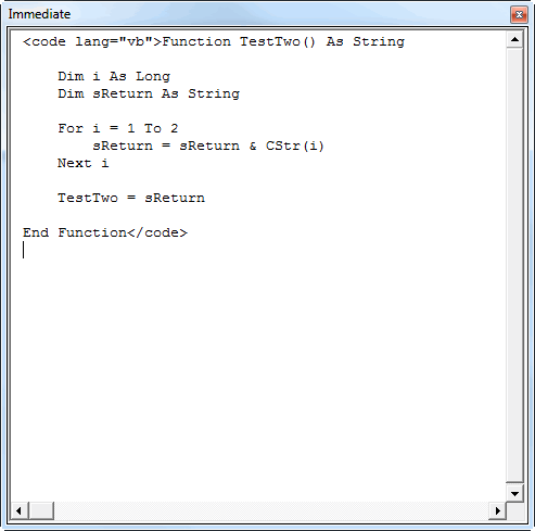
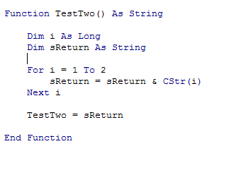
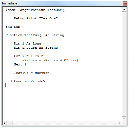
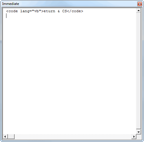
For years I’ve been typing <code> tags and pasting code between them. But no more! I wrote a small utility that puts the code tags around my code and pops into the clipboard. Think of the seconds that I’ll save.

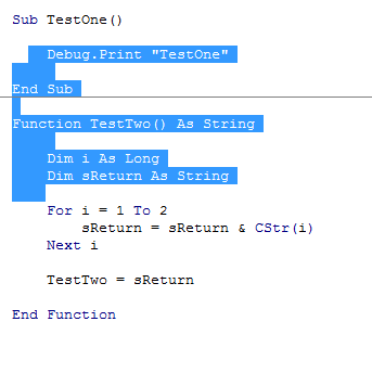
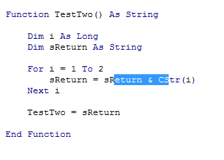
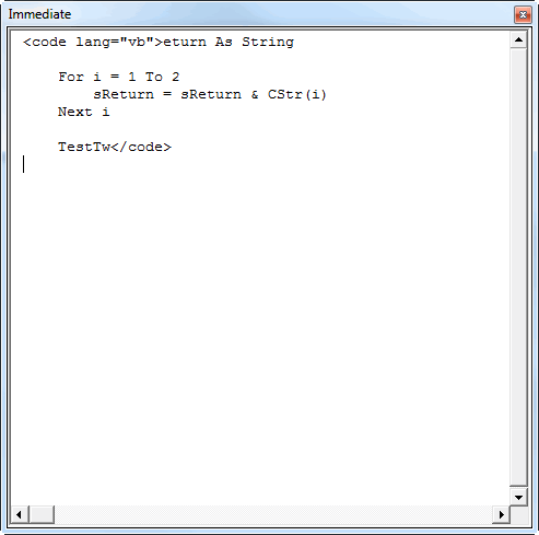
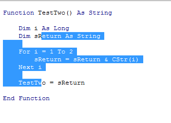
There are three situations that I wanted to cover with this code; no selection, multiple procedure selection, and intra-procedure selection. If there’s no selection, I want the whole procedure that contains the cursor. If the selection spans more than one procedure, I want the entirety of all the procedures that are touched by the selection. If the selection is within one procedure, I want what’s selected.

This code uses the Microsoft Visual Basic Extensibility library.

To get this	Select this

Sub CreateCodeTags()



Dim cp As CodePane, cm As CodeModule

Dim lStartLine As Long, lEndLine As Long

Dim lStartCol As Long, lEndCol As Long

Dim sStartProc As String, sEndProc As String

Dim lStartType As Long, lEndType As Long

Dim sOutput As String

Dim doClip As DataObject



Set cp = Application.VBE.ActiveCodePane

Set cm = cp.CodeModule



cp.GetSelection lStartLine, lStartCol, lEndLine, lEndCol



sStartProc = cm.ProcOfLine(lStartLine, lStartType)

sEndProc = cm.ProcOfLine(lEndLine, lEndType)



‘Single cursor = get whole procedure

If lStartLine = lEndLine And lStartCol = lEndCol Then

sOutput = cm.Lines(cm.ProcStartLine(sStartProc, lStartType) + 1, cm.ProcCountLines(sStartProc, lStartType) – 1)

‘Spans more than one procedure = get all procedures in selection

ElseIf sStartProc <> sEndProc Then

lStartLine = cm.ProcStartLine(sStartProc, lStartType) + 1

lEndLine = cm.ProcStartLine(sEndProc, lEndType) + cm.ProcCountLines(sEndProc, lEndType)

sOutput = cm.Lines(lStartLine, lEndLine – lStartLine)



‘Same line = get selected text

ElseIf lStartLine = lEndLine Then

sOutput = Mid$(cm.Lines(lStartLine, 1), lStartCol, lEndCol – lStartCol)



‘Multiple lines = get selected text

Else

sOutput = Mid$(cm.Lines(lStartLine, 1), lStartCol, Len(cm.Lines(lStartLine, 1)))

If lEndLine – lStartLine > 1 Then

sOutput = sOutput & vbNewLine & cm.Lines(lStartLine + 1, (lEndLine) – (lStartLine + 1))

End If

sOutput = sOutput & vbNewLine & Left$(cm.Lines(lEndLine, 1), lEndCol – 1)

End If



If Right$(sOutput, Len(vbNewLine)) = vbNewLine Then

sOutput = Left$(sOutput, Len(sOutput) – Len(vbNewLine))

End If



sOutput = “< code lang=”“vb”“>” & sOutput & “< /code>”



Set doClip = New DataObject



doClip.SetText sOutput

doClip.PutInClipboard



End Sub

In the last line that begins with

<span class="vb">sOutput =</span>

I had to add some extraneous spaces to be able to post code that contains code tags, but they’re not really there in the code.

Other than that I’m merely doing string manipulation with my starting and ending lines and columns.

I think I need to add the

<span class="text">inline = "true"</span>

argument when I’m on a single line. I think I’ll use and see how often I’m adding it.

Display Contact Group Member Count

From : Code For Excel And Outlook - Learn VBA »

Display Contact Group Member Count:

Sorry for the lack of posts lately. I've been working on the next version of Random Data Generator, and my home network connection wasn't working for the past few days.

In Display the Total Number of Members in a Contact Group there is a method for displaying the number of members of a contact group (aka distribution list).

There is an easier way, using VBA:

Sub GetDistListCount()

Dim dl As Outlook.DistListItem

Set dl = ActiveExplorer.Selection.item(1)

MsgBox "There are " & dl.MemberCount & " member(s) in this contact group."

End Sub

Just go to your Contacts folder, select a distribution list item and run this code. There is no error handling here, just a simple procedure to display the number of members of the group.

Related Articles:

• June 23, 2011 -- Manage your email overload
• March 7, 2011 -- Get Word Count in VBA
• January 31, 2011 -- Add photos to Contacts in bulk using VBA in Outlook

Display Contact Group Member Count is Copyright © Code For Excel And Outlook - Learn VBA. All Rights Reserved.

Help with Compile error Next without for

From ExcelExpert.com

Help with Compile error Next without for: I'm trying to get excel to send an email when a command button is pushed. The email needs to be sent out if any date in column E equals today's date. I keep getting a compile error Next without for. Here's the Macro

Sub SendEmail()
'Uses early binding

Dim OutlookApp As Object
Dim MItem As Object
Dim Today As Object
Dim cell As Range
Dim Subj As Variant
Dim EmailAddr As String
Dim Scie As String
Dim CnNo As String
Dim Msg As String
'Create Outlook Object
On Error GoTo debugs
Set OutlookApp = CreateObject("Outlook.Application")
Set Today = cell.Value("C1")
'Loop through the rows
For Each cell In Columns("E").Cells.SpecialCells(xlCellTypeConstants)
 With cell.Value = Today
 'Get the data
  Subj = "Please check the CN Tracker, a CN has been assigned to you "
 Scie = cell.Offset(0, 8).Value
 EmailAddr = cell.Offset(0, 9).Value
 CnNo = Format(cell.Offset(0, -3).Value, "0,000.")
 'Compose message
  Msg = "Dear " & Scie & vbCrLf & vbCrLf
 Msg = Msg & "CN " & CnNo & " has been assigned to you. " & vbCrLf & vbCrLf
 Msg = Msg & "Please check the CN tracker and request the technical solution and supplier contact information from the responsible engineer. " & vbCrLf & vbCrLf
 Msg = Msg & "Have a great day. " & vbCrLf & vbCrLf
 Msg = Msg & " " & vbCrLf & vbCrLf
 Msg = Msg & " " & vbCrLf & vbCrLf
 Msg = Msg & "************This is an automated message, please do not. **************"
 'Create Mail Item and send it
  Set MItem = OutlookApp.CreateItem(olMailItem)
 With MItem
  .To = EmailAddr
  .Subject = Subj
  .Body = Msg
  .Send
    End With
debugs:
If Err.Description <> "" Then MsgBox Err.Description
Next
End If
End Sub
Private Sub CommandButton1_Click()
Sheet1.SendEmail
End Sub

What am I missing?

If Err.Description <> "" Then MsgBox Err.Description   RESUME Next End If

Add Data to Charts with Copy Paste [Quick Tip]

From Chandoo.rog

Add Data to Charts with Copy Paste [Quick Tip]:

So how did your weekend go?

I did a bit of gardening, painted our car shed, played badminton (I am learning), attended 60th birthday of a close friend’s dad. Pretty hectic, but fun as usual.

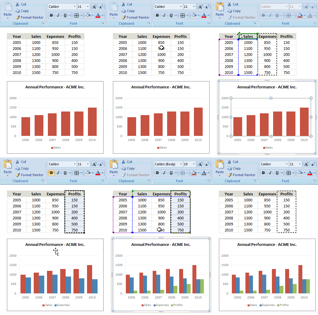
To start this week, let me share a simple but fun way to add data to charts.

Lets say you have a chart that depicts Annual sales for last few years. And you want to add the data of Profits (or Expenses) to this chart. Here is a dead-simple way to do it.

1. Copy the profit data by selecting it and pressing CTRL+C


2. Select the chart


3. Paste by pressing CTRL+V


4. That is all!

See the demo alongside to understand how this works.

Bonus Tips:

1. While pasting, if you go for Paste Special (CTRL+ALT+V or ALT+E S) you can tell whether the data should be added as a new series or new points and several other things.


2. To remove a series of data from a chart, just select the series and hit DEL key.


3. To extend a series (ie add new points to it), select the series. Now you will see that Excel has highlighted the range of cells corresponding to that series. Just point your mouse at the bottom-right corner and resize the range to add new points to the chart.

More Quick Tips on Excel Charting

There are a ton of things you can do in Excel with a click of mouse or press of few keys. Whenever we learn something that is simple yet very useful, we share it as a quick tip. Browse thru these to learn more on Excel Charting.

• Highlight points in line charts & scatter plots


• Display Alert Symbols in Dashboards using Conditional Formatting


• Change Data Labels in Charts to whatever you want


• Use Paste Special to Speed up Chart Formatting


• Hide “0″ in Excel Chart’s Axis


• Create a combination chart, add secondary axis


• More Quick Tips & Chart Formatting Tips

（未知标题）

From Chandoo.org

（未知标题）:

Last week Joyce asked a question on the Chandoo.org, Comment 24.

I’m wondering if there’s a way to count the number of occurrences of words when they’re all in a cell? Like this:

A1: “Windows NT, Networking, Firewalls, Security, TL, Training”

A2: “Networking, Networking, Training, Security, TL, Training”

A3: “Security, TL, Firewalls, Security, Networking, Windows NT”

Hui responded with an Array Formula:

=SUM(LEN(A1:A3)-LEN(SUBSTITUTE(A1:A3,C10,””)))/LEN(C10)

As the formula is an Array Formula it is entered with Ctrl Shift Enter.

Setup the Problem

Copy the Data Above into Cells A1:A3 or download the example file here: Example File

Enter the value Security into cell C10

And array enter the formula

D10: =SUM(LEN(A1:A3)-LEN(SUBSTITUTE(A1:A3,C10,””)))/LEN(C10)

Pull The Formula Apart

Lets take a look inside this and see how it works

We will break this formula apart and look at each section independently and then put the answers back together.

=SUM(LEN(A1:A3)-LEN(SUBSTITUTE(A1:A3,C10,””)))/LEN(C10)

In a cell below the data

D13: =LEN(A1:A3) but don’t press Enter, Press F9

Excel displays ={57,56,57}

This is the number of characters in each cell A1:A3

ie: A1 has 57 characters, A2 has 56 characters, A3 has 57 characters,

=SUM(LEN(A1:A3)-LEN(SUBSTITUTE(A1:A3,C10,””)))/LEN(C10)

In another cell below the data

D15: =LEN(SUBSTITUTE(A1:A3,C10,”")) but don’t press Enter, Press F9

Excel displays ={49,48,41}

What this section does is measure the length of each cell in A1:A3 but only after substituting the word being searched for from C10 with ””, which is a zero length string.

So the second array is shorter by X times the length of the word in C10

=SUM(LEN(A1:A3) – LEN(SUBSTITUTE(A1:A3,C10,””)))/LEN(C10)

Next we add up the difference between the two arrays

So you can see we have two arrays of numbers

Array 1 = {57,56,57}

Array 2 = {49,48,41}

If we subtract Array 2 from Array 1

= {57-49, 56-48, 57-41}

= {8, 8, 16}

We can do this in Excel to Check

In Cell D17 enter

=LEN(A1:A3)-LEN(SUBSTITUTE(A1:A3,C10,”")) and press F9

Excel displays: = {8, 8, 16}

=SUM(LEN(A1:A3) – LEN(SUBSTITUTE(A1:A3,C10,””)))/LEN(C10)

The next part is to sum these up

Obviously the sum of 8, 8 & 16 is 32

We can check that

D21: =SUM(LEN(A1:A3)-LEN(SUBSTITUTE(A1:A3,C10,”"))) and press F9

Excel displays: 32

=SUM(LEN(A1:A3) – LEN(SUBSTITUTE(A1:A3,C10,””)))/LEN(C10)

The final part of this is to divide the sum (32 in this case) by the length of the text in C10 “Security” = 8 Characters

=32 / 8

= 4

OTHER POSTS IN THIS SERIES:

You can learn more about how to pull Excel Formulas apart in the following posts

Formula Forensic 001 – Taruns Problem

WHAT FORMULAS WOULD YOU LIKE EXAMINED

If you have any formulas you would like explained please feel free to leave a post here or send me an email:

If the formula is already on Chandoo.org or Chandoo.org/Forums, simply send the link to the post and a Comment number if appropriate.

If sending emails please attach an Excel file with the formula and data

A Technique to Quickly Develop Custom Number Formats

From Chandoo.org

A Technique to Quickly Develop Custom Number Formats:

In the past Chandoo has written about custom Number Formats for cells:

http://chandoo.org/wp/2008/02/25/custom-cell-formatting-in-excel-few-tips-tricks/

http://chandoo.org/wp/tag/custom-cell-formatting/

and I have written about Custom Number Formats for Charts:

http://chandoo.org/wp/2011/08/19/selective-chart-axis-formating/

http://chandoo.org/wp/2011/08/22/custom-chart-axis-formating-part-2/

This post examines a technique for quickly developing Custom Number Formats for Cells, Charts or any other Number location in Excel.

A Technique for Quickly Developing Custom Number Formats

Instead of Selecting the cell, chart axis etc, Ctrl 1, Format Cells/Properties, Number Tab, Custom and then entering a Custom Format and Apply, only to find out that the format is incorrect, try this simple technique below.

1. Enter a few Numbers in 3 cells

Enter 3 numbers, a positive, zero and negative which have values you will expect to receive in your model.

2. Add a Custom Format Cell

In D3 I have entered ##,;-(##,);”Zero”

3. Display Numbers using the custom Format

Each Number to a display cell with a simple =Text(B3,$D$3)

Copy down

This will display the 3 numbers using the Custom Format in Cell D3

4. Develop Your Custom Format

Play around with your own Custom Number Formats to your hearts content

5. Use your new format

Once you have completed your new Custom Number Format, copy the cell contents of D3 in this case.

Select your cells/or other Excel Numbers,

Ctrl 1,

Format Cells/Properties,

Number Tab, Custom

Enter the Custom Format and Apply.

6. Extending the Technique

This technique can be extended by adding several more rows with a larger range of values.

The values are all evaluated at the same time

LIMITATIONS

The above technique does not show the effects of the Color Modifiers in the test cells

But I think it is a safe bet that you will understand what the Modifier [Red] will do

There are also reserved characters such as E

So in the above example if I had used Zero instead of “Zero”

It would have displayed Ze1900ro, where the E in Zero is taken as 10^x and x=0 so Excel interprets e as 0 or 1900, a date?

You can avoid this by using the code “Zero” or Z\ero

DOWNLOAD

You can download the worked Example File used above.

NUMBER FORMATS

For more on Number Formats check out the above links or those below:

http://www.ozgrid.com/Excel/excel-custom-number-formats.htm

http://www.ozgrid.com/Excel/CustomFormats.htm

http://peltiertech.com/Excel/NumberFormats.html

How to Look up Based on Multiple Conditions

From chandoo.org

How to Look up Based on Multiple Conditions:

This article is part of our VLOOKUP Week. Read more.

Situation

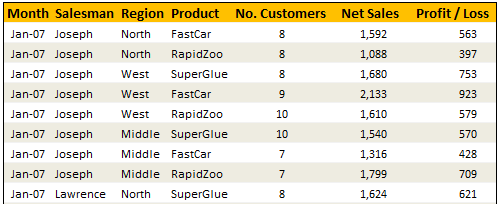
Not always we want to lookup values based on one search parameter. For eg. Imagine you have data like below and you want to find how much sales Joseph made in January 2007 in North region for product “Fast car”?

Data:

Solution

Simple, use your index finger to scan the list and find the match

Of course, that wouldn’t be scalable. Plus, you may want to put your index finger to better use, like typing . So, lets come up with some formulas that do this for us.

You can extract items from a table that match multiple criteria in multiple ways. See the examples to understand the techniques:

Using SUMIFS Formula [help]
Formula	=SUMIFS(lstSales, lstSalesman,valSalesman, lstMonths,valMonth, lstRegion,valRegion, lstProduct,valProduct)
Result	1592
Using SUMPRODUCT Formula [help]
Formula	=SUMPRODUCT(lstSales,(lstSalesman=valSalesman)*(lstMonths=valMonth)*(lstRegion=valRegion)* (lstProduct=valProduct))
Result	1592
Using INDEX & Match Formulas (Array Formula) [help]
Formula	{=INDEX(lstSales,MATCH(valSalesman&valMonth&valRegion&valProduct, lstSalesman&lstMonths&lstRegion&lstProduct,0))}
Result	1592
Using VLOOKUP Formula [help]
Formula	=VLOOKUP(valMonth&valSalesman&valRegion&valProduct,tblData2,7,FALSE)
Result	1592
Conditions:	A helper column that concatenates month, salesman, region & product in the left most column of tblData2
Using SUM (Array Formula) [help]
Formula	{=SUM(lstSales*(lstSalesman=valSalesman)*(lstMonths=valMonth)* (lstRegion=valRegion)*(lstProduct=valProduct))}
Result	1592

Sample File

Download Example File – Looking up Based on More than One Value

Go ahead and download the file. It also has some homework for you to practice these formula tricks.

Also checkout the examples Vinod has prepared.

Special Thanks to

Rohit1409, dan l, John, Godzilla, Vinod

Similar Tips

• Excel SUMIFS Formula – What is it, how to use it & examples


• Excel SUMPRODUCT Formula – What is it, how to use it & examples