Simple KPI Dashboard using Excel

From Chandoo.org

Simple KPI Dashboard using Excel:
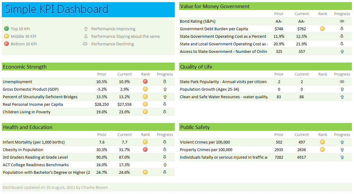
Any Tom, Dick and Sally can make things complex. It takes guts and clarity to simplify things. That is why I was pleasantly surprised to see this dashboard prepared by Michigan State. You can see it below:



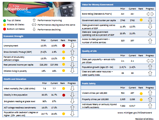
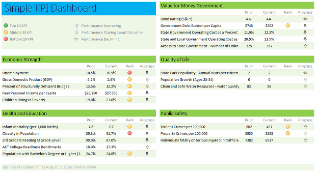
Linda, one of My Excel School students shared this dashboard link with me and asked if I can show how to construct something like this. Here is my version of the dashboard.

[Click here for larger version]

There are 2 parts in construction of a dashboard like this.

1. Defining the vision, layout & metrics that you want.


2. Creating the dashboard in Excel (or any other tool)

While it does not seem so, it is the Step 1 that takes a lot of time and hard-work.

Step 1: Defining the dashboard metrics, layout & vision

This is the most time consuming part of any dashboard. There is no one way to do this step. So I am going list a set of guidelines for you to follow.

• Speak with your audience & define what they want: For any dashboard, you will have some audience. So speak with them, understand what their information needs are. List down everything they want to know. Some parameters you want to consider are,
  
  
  
  • Metrics / KPI they are interested
  
  
  • Frequency of the need (weekly, monthly or yearly etc.)
  
  
  • Granularity of the information (example: person level, department level, company level)
  
  
  • Type of the need (information, analytical, mission critical etc.)


• Understand the sources of data: Another tricky part of a dashboard development is to get right data. In corporate environments, your data sources may be spread across and follow their own formats. So you need to plan ahead for all these differences, otherwise, you will end up doing lots of extra work.


• Prioritize the information: Once you have listed down various metrics, KPIs, information pieces to be used in the dashboard, list them down in the order of priority. Metrics or KPIs that are most important and indicate the overall health of the system (or project, initiative or company) should be on top.


• Remove ruthlessly: Now comes the tricky part. You must remove items, metrics and information that is low on value from the end dashboard. This is where your persuasion, negotiation skills come in handy.


• Make a rough sketch of the dashboard: Even before you make something in Excel, just make a rough sketch using pen and paper (or MS Paint or PowerPoint). This way, you can validate the design with end users and get buy-in early. (related: use excel for screen prototyping)

There are more ideas and tactics you can follow. But if you follow the above guidelines, then 80% of your work is done.

Step 2: Designing Excel Dashboard

This step becomes easier once you have clarity of vision and listed down what you want (and what you dont want). And if you find this difficult, there is always help.

In this, let us learn how to construct the particular dashboard you see above.

1. Arrange the data: For a simple dashboard like this, you can arrange the data in this fashion.
   
   


2. Create Dashboard Layout and Load data: Once the data is in-place, create a blank layout. You can follow any template. I liked the Michigan State Dashboard template and created something like that.
   
   Once the layout is ready, link to the source data (using Copy & Paste as links).
   
   


3. Use Conditional Formatting & Formulas to Display Icons: Once the data is loaded, next step is to show icons. This can be done easily with Conditional Formatting and simple formulas. (tip: display alerts in dashboards using conditional formatting)


4. Format: Now format everything so it looks awesome.

That is all. You are done!

Download Simple KPI Dashboard Workbook

Click here to download the workbook & play with it.

Special thanks to Michigan State website for the inspiration & Linda for sharing the link.

Do you like this dashboard?

I really liked the simplicity of this dashboard. The Michigan state government folks have done fine job of listing down the metrics and carefully capturing them and presenting the outlook in a crisp fashion.

What about you? Do you like the ideas shared in this article? How would you approach a dashboard project? Please share your tips & ideas using comments.

Want to Learn Dashboards? Go thru these resources:

If you want to learn dashboards, then you have come to the right place. Click thru below links to access a ton of information, ideas & material.

• KPI Dashboards in Excel – 6 part tutorial


• Project Management Dashboard in Excel


• Sales Dashboards in Excel


• More on Dashboards


• Join our Excel School Dashboards Program

Table of Contents for Long Excel Sheet

From http://blog.contextures.com/

Table of Contents for Long Excel Sheet:

In the comments for my post on creating a table of contents in Excel, Eden asked:

“Can I create a content page within one worksheet? I have one worksheet and it is very long.”

Good idea! A short table of contents at the top of a worksheet would make it easy to find specific sections on a long worksheet. Here are the steps for setting that up.

Create the Headings List

The first step is to copy all the headings to the top of the worksheet, where they’ll be used for the table of contents.

1. Insert blank rows at the top of your worksheet, to make room for the table of contents.


2. Click on the first heading, to select it.


3. Press the Ctrl key, and click on each of the remaining headings, to select all of them.


4. Click the Copy command on the Excel Ribbon


5. Right-click in an empty cell at the top of the worksheet, and under Paste Options, click Paste as Values

That creates a list of headings at the top of the sheet.

Name the Heading Cells

Next, follow these steps, to create a named range for each heading cell.

1. In the body of the worksheet, select the cell with the first heading.


2. To name that cell, click in the name box, to the left of the Formula Bar.


3. Type a short one-word name for that range, and press Enter.


4. Repeat these steps, to name each of the remaining headings.

In this example, the first heading cell is named Income.

Add Links in the Table of Contents

The final step is to link the headings to the table of contents, by following these steps.

1. At the top of the worksheet, select the cell with the first heading that you’re going to link.


2. On the Excel Ribbon’s Insert tab, click Hyperlink


3. Under Link To, click on Place in This Document


4. Under Defined Names, click on that heading name – Income in this example.


5. (Optional) Click Screen Tip, and type the heading name, then click OK


6. Click OK, to close the Insert Hyperlink dialog box.

Now you have a list at the top of the worksheet that’s linked to each of the sections below.

Link to the Links

To make navigation even easier, you could put a link near each of the subheadings, to take you back to the table of contents.

• First, name a cell at the top of the worksheet. In the screen shot below, the main heading cell is named TopSummary

• Next, add a shape to the worksheet, to the left of the first heading cell. I added a small arrow, and set its properties to not Print, and Move, but don’t Size with cell.

• With the shape selected, insert a Hyperlink to the named range at the top of the sheet.

Copy the shape, and paste to the left of the remaining headings.

Test the Navigation

Now your navigation system is ready to test.

1. Click on a link in the table of contents to quickly go to a section in the report.


2. Click on an arrow, to return to the top of the worksheet.

Did it work? Do you have any other ideas for navigating through a long worksheet? Please let me know in the comments!

___________

Change Name in Excel Comments

From http://blog.contextures.com/

Change Name in Excel Comments:

When you add a comment to an Excel worksheet, your name is added at the top of the comment. Your name also appears in the status bar, when you point to the cell that contains the comment.

It’s nice to be recognized, but sometimes you want to change the name that appears. For example, maybe you were working on the file for a client, and now you want to put the client’s name in the comments, instead of your own.

Keep reading, to see how you can quickly change the names with a macro, and see how that macro works.

How the Replace Comment Name Macro Works

In this sample file, there is a macro that replaces the old comment names, with a new name.

First, the macro prompts you for the old name – by default, the current User Name is entered.

Next, you’ll enter the new name for the comments. You can’t leave this blank – enter at least one character, even if it’s a space character.

The replaces the current User Name with the New Name. Then, it deletes each existing comment, and replaces it with a new comment. That changes the name in the status bar.

When the new comment is inserted, the Old Name at the top is replaced with the New Name.

At the end of the macro, you can decide if you want to keep the new name as the User Name for Microsoft Office.

• Click No, if you want to keep your current user name. In this example, I want to replace the comment names in a file for my client. At the end of the macro I’d click No, because I don’t want to change the User Name on my computer – just the comment names.


• If you want to keep the New Name as the User Name, click Yes.

Now, when you point to a cell with a comment, the New Name appears in both the comment, and the status bar.

Excel VBA Code to Replace Comment Name

To quickly change the name that appears in the status bar and the comment, you can use the following Excel VBA code.

If you’re not sure what comment names are in the workbook, you can create a list of Excel comments, with their details. Then, run this Change Comment Name code – more than once, if there are multiple old names.

For more comment programming examples, see Excel Comments VBA.

Sub ChangeCommentName()

'downloaded from www.contextures.com

'replaces old names in comments

'deletes and reinserts comments,

'so new name appears in status bar



Dim ws As Worksheet

Dim cmt As Comment

Dim cmt2 As Comment

Dim strOld As String

Dim strNew As String

Dim strUser As String

Dim strComment As String

Dim strMsg As String

Dim lBreak As Long

Dim bUser As Boolean



On Error GoTo errHandler



strUser = Application.UserName



strOld = InputBox("Old Name", "Replace Comment Name", strUser)

If Len(strOld) = 0 Then

 strMsg = "Cannot change comment names" _

     & vbCrLf _

     & "Old name must be at least one character"

 GoTo exitHandler

End If



strNew = InputBox("New Name (at least one character)", "Replace Comment Name", strUser)

If Len(strNew) = 0 Then

 strMsg = "Cannot change comment names" _

     & vbCrLf _

     & "New name must be at least one character"

 GoTo exitHandler

End If



Application.UserName = strNew

strMsg = "Could not change comments"



For Each ws In ActiveWorkbook.Worksheets

For Each cmt In ws.Comments

 strComment = Replace(cmt.Text, strOld, strNew)

 cmt.Delete

 Set cmt2 = cmt.Parent.AddComment

 cmt2.Text Text:=strComment



 lBreak = InStr(1, cmt2.Text, Chr(10))

 If lBreak > 0 Then

   With cmt2.Shape.TextFrame

     .Characters.Font.bOld = False

     .Characters(1, lBreak - 1).Font.bOld = True

   End With

 End If

Next cmt

Next ws



bUser = MsgBox("Keep New Name as User Name?", vbYesNo + vbQuestion, "Excel User Name")

If bUser <> vbYes Then

 Application.UserName = strUser

End If

strMsg = "Done!"



exitHandler:

 MsgBox strMsg

 Exit Sub

errHandler:

 Resume exitHandler



End Sub

______________

10 Excel Keyboard Shortcuts I can’t live without!

From http://chandoo.org/wp

10 Excel Keyboard Shortcuts I can’t live without!:

Everyone and their colleague knows the importance of Excel keyboard shortcuts. While it may be a good idea to know a 97 different shortcuts for everything in Excel, the fact is, you don’t use them all the time. So, it all boils down to memorizing the few shortcuts that you use all the time.

In this post, I am sharing 10 such shortcuts that I can’t live without, especially, when I am analyzing data, making charts and formatting my workbooks.

1. CTRL+1 – Format

Oh CTRL+1, if I get an ear, every-time I press you, I would be a millionear by now.

I use this all the time, to format cells, charts, text boxes – you name it.

2. CTRL+SHIFT+L – Turn on/ off filters

Most of the time, I use filters to do ad-hoc analysis of my data. So, Once I set a couple of filters, If I want to revert back to full data, I find clearing each filter a pain. So I just turn-off and turn-on the filters, by pressing CTRL+SHIFT+L twice.

3. CTRL+Arrow keys – Navigate around the workbook

When it comes to dealing with data, navigate, you must. So I rely on CTRL+arrow key combinations all the time. Also, I use CTRL+SHIFT+arrow keys to select a group of cells

4. ALT+ES – Paste Special > Values

Copying and Pasting is another must if you deal with data. Often, I have to get data from other workbooks or clean the formatting of existing tables. So I use ALT+ES (press E then leave the key and press S) to paste special. Works like a charm! [more: 16 more paste special tricks]

5. F4 – Change cell reference style while editing formulas

Excel runs a pretty tight mafia when it comes to cell references. You must pay it a couple of $s if you want to change the reference style from relative (A2) to absolute ($A$2). But whos got the time to carefully navigate between A and 2 and then type SHIFT+4? So I use F4 key and Excel changes the referencing style for me. [More: Relative vs. Absolute Cell References in Excel]

6. F2 – Edit a cell

As simple as that.

7. F3 – Show Names

For simple workbooks I do not use names. But if I am making a dashboard or Excel model, I define several names and use them all the time. This is where F3 comes in handy. Just press F3, no matter where you are (formula editing, conditional formatting, data validation etc.) and you get a list of all the defined names. Pick one and press ok to add it to the formula etc. you are typing.

8. CTRL+K – Add Hyperlink

Hyperlinks make your work book accessible & pretty. So I use them all the time, especially, if I have more than a couple of sheets. Select a cell or shape and press CTRL+K to launch hyperlink box. Type the destination URL or location and you are done.

9. CTRL+T – Insert Table

Ever since I learned how to use Tables feature, I have never looked back. Nowadays, anytime I need to use a bunch of data, I convert that to a table and then use. Tables are flexible, they can grow & shrink, they allow you to write readable formulas (structural references) and they are lovely. Just select any cell in a range of related data, and press CTRL+T to make it table.

10. CTRL+S – Save

There is no point making something elaborate in Excel if you forgot to save. So I press CTRL+S every now and then. You never know when aliens strike!

What are the keyboard shorts you cannot live without?

Now your turn. Go ahead and share the list of shortcuts you use everyday. And if you do not use keyboard shortcuts at all, its about time you started. You can save a lot of time and effort. Time you can use to do other fun things like leaving comments on our website

Go ahead and share.

Learn more keyboard shortcuts:

I love keyboard shortcuts & productivity tricks. So, naturally, we have a lot of articles on the same. Go thru the below stuff to one up your Excel mojo, seriously!

• Excel Keyboard Shortcuts – a comprehensive list


• Do you know these Excel Productivity Secrets?


• Save time & be awesome by double clicking in Excel


• Learn how to master Excel Ribbon [FREE PDF Guide]


• More productivity tips & keyboard shortcuts

Sumproduct function to Consolidate Revenues?

From Chandoo.org

Sumproduct function to Consolidate Revenues?: "

Chandoo.org is all about simplifying life using Excel. When I first started visiting the site, I was amazed at the amount of information on the site, which made your life easier. My next few posts would be about excel functions which can make your life for Financial Modeling easier! These are simple examples that you might find relevant in your daily life as well.

Let’s say your organization had 10 business segments, each segment selling different products at different prices. You have data available for the segments, how do you consolidate the revenues in one shot?

How do you model this in excel fast? In this tutorial we understand how you can use SumProduct() formula to do that!

What is the SumProduct() function

SumProduct() formula in excel, would take a couple of arrays (Say A and B) as inputs. Multiple corresponding items in each Array – A[1] x B[1], A[2] x B[2], … and sum them together.

SumProduct would get you the total revenue from a segmental breakup

The function is simple, it does all the difficult calculations for you and gets you the solution!

Traditional way of calculating consolidated Revenues

Step I: Getting the Segmental Revenues

Step II: Summing up the revenues

Consolidated Revenues using SumProduct()

Using the SumProduct() the consolidated revenues can be calculated in a single cell! It’s like the calculation is on fire!

Where else can this function be useful in Finance?

The function would see a lot of usage in the financial models. You can use it to consolidate revenues (Segmental volumes and prices to total revenues), calculate depreciations (when you have various assets and depreciation rates), consolidate costs (different raw material prices and volumes), NPV (Discount Rates and Cash flows), etc.

Are you also using SumProduct() function in Finance?

I have used SumProduct in my models. I find them to be very useful and speed up the modelling process. But sometimes I find that they confuse the readers of my model. Have you used the function in your models?

Templates to download

I have created a template for you, where the subheadings are given and you have use the functions to get the right values for you! You can download the same from here. You can go through the case and fill in the yellow boxes. I also recommend that you try to create this structure on your own (so that you get a hang of what information is to be recorded).

Also you can download this filled template and check, if the information you recorded, matches mine or not!

Join our Financial Modeling Classes

We are glad to inform that our new financial modeling & project finance modeling online class is ready for your consideration.

Please click here to learn more about the program & sign-up.

The article is written by Paramdeep from Pristine.

Chandoo.org has partnered with Pristine to launch a Financial Modeling Course. For details click here.

"

Shift Calendar Template – FREE Download

From http://chandoo.org/wp

hift Calendar Template – FREE Download: "

Today I want to share an Employee Shift Calendar Template with you. You can use this template to keep track of shift timings on various days.

See a demo of the template:

How does this template work?

This template uses a 3 main ideas,

• Excel formulas to create the calendar & checking for a day’s shift


• Conditional formatting to highlight a date in different color based on shift


• Scroll-bar form control to change the month

Here is a brief illustration explaining how this template works:

For more information on these techniques visit,

• Building a Calendar in Excel


• VLOOKUP formula – Introduction & uses


• Conditional formatting – Introduction & tutorial


• Form Controls in Excel – What are they and how to use them?


• Range lookup in Excel – how to write formulas?

Download Excel Template for Employee Shift Tracking & Shift Calendar

Download the Employee Shift Tracking Template

Go ahead and play with the file to learn more.

How to use this template?

I made a short video explaining this template and how to use it. See it below (or on our YouTube Channel).

Do you like this template?

I like the challenge of building this template. It nicely integrates 3 powerful ideas – date formulas, conditional formatting & form controls to create a concise tracker to manage employee shift data.

What about you? Did you like this template? How are you planning to use it? Please share using comments.

More templates & downloads

We got more templates to make you awesome!!! Go ahead and try these and impress someone.

• New year resolutions template in Excel


• Holiday (Vacation) Request Form Template


• Free 2011 Calendar Template (secret: works for any year too)


• Annual Goal Tracker Template


• Expense Trackers


• Project Management Templates [for sale]

PS: Thanks to Denice, who emailed me and asked for this template.

"