Prevent Spaces in Excel Data Entry Cell

From Contextures Blog

Prevent Spaces in Excel Data Entry Cell:
In Excel, you can use data validation to control (to some extent!) what users can enter in a cell. One option is to create a drop down list, so users can only select from a list of valid options.

Data Validation Custom Criteria

In some cases, a drop down list isn’t practical, but you still want some control over what goes into the cell. For example, in the screen shot below, we want to prevent users from typing a space character in the cell.



To do this, you can use data validation with custom criteria. Thanks to Jerry Latham for sending this example, and the custom validation formula.

Follow these steps to set up the data validation.

• Select cell B3, where the item code, with no spaces, will be entered.


• On the Excel Ribbon, click the Data tab, and click Data Validation


• In the Data Validation dialog box, on the Settings tab, select Custom


• In the formula box, type this formula, which refers to the active cell (B3), then click OK
  
  
  
  • =B3=SUBSTITUTE(B3," ","")

How It Works

The SUBSTITUTE function replaces each space character – " " – with an empty string – ""

The value entered in cell B3 must be equal to the result of that SUBSTITUTE function. If there is a space in B3, the results won’t be equal, so the data validation test will fail.

For more examples of Custom data validation, see the Data Validation Custom Criteria Examples page on the Contextures website.

________________

Sum of Values Between 2 Dates [Excel Formulas]

From chandoo.org

Sum of Values Between 2 Dates [Excel Formulas]:

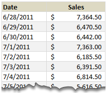
Lets just say, you run a nice little orange shop called, “Joe’s Awesome Oranges“. And being an Excel buff, you record the daily sales in to a workbook, in this format.

After recording the sales for a couple of months, you got a refreshing idea, why not analyze the sales between any given 2 dates? for analysis sake.

So you entered 2 dates, Starting Date in cell F5 and Ending Date in cell F6

How would you sum up the sales between the dates in F5 & F6?

This is where use the powerful SUMIFS formula.

Assuming the dates are in column B & sales are in column C,

we write =SUMIFS($C$5:$C$95,$B$5:$B$95,">="&$F$5,$B$5:$B$95,"<="&$F$6)

to calculate the sum of sales between the dates in F5 & F6.

How does this formula work?

• $C$5:$C$95 portion: This is the range of cells where our Sales values are recorded. We want these to be summed up based on the conditions as below.


• Condition 1: $B$5:$B$95 >= $F$5: This condition tells SUMIFS to check Column B for any dates on or after F5


• Condition 2: $B$5:$B$95 <= $F$6: This condition tells SUMIFS to check Column B for any dates on or before F6


• When combined, the SUMIFS formula checks for both conditions and adds sales only for dates between Starting (F5) and Ending (F6) dates.


• Learn more about SUMIFS syntax & how to use it.

What formula you should use in Excel 2003?

As you may know, SUMIFS formula does not work in earlier versions of Excel. But you don’t have to shut your orange shop because of that. We can use the all powerful SUMPRODUCT formula for this.

For example, =SUMPRODUCT(($B$5:$B$95>=$F$5)*($B$5:$B$95<=$F$6),$C$5:$C$95) would work the same.

Learn more about SUMPRODUCT formula & why it is awesome.

We can even use SUM & OFFSET formulas if …,

We can also use SUM & OFFSET combination to perform this calculation, provided dates are in smallest first order and all dates are entered. For the example, see download file.

Download Example Workbook:

Click here to download example workbook & play with it.

How would you sum up values between 2 dates?

In reporting situations, showing summary of values between 2 dates is a common requirement. So I use either formulas like above or Pivot Tables to do this.

What about you? How would you sum up values between 2 dates? Please share your ideas & tips using comments.

Learn More Date Related Formulas:

• How to find if 2 sets of dates overlap?


• Extract Quarterly Totals from Monthly Data


• Automatic Rolling Months in Excel


• How to Clean-up Dates in Excel


• Calculate Elapsed Time in Excel


• More on Date & Time

Want to Learn More Formulas? Join Our Crash Course

If you want to learn SUMIFS, SUMPRODUCT, OFFSET and 40 other day to day formulas, then consider my Excel Formula Crash Course. It has 31 lessons split in to 6 modules and makes you awesome in Excel formulas.

Click here to learn more about this.

Saving/Deleting All Attachments With One Click

from http://techniclee.wordpress.com

Saving/Deleting All Attachments With One Click:

This post is in response to a tweet from petemarcus that was retweeted by malcolmcoles. Here’s what petemarcus said:

Dull tweet alert. Microsoft Outlook needs a ‘remove all attachments’ button as well as ‘save all’. Good to get that off my chest.

While Pete and Malcolm wait for Microsoft to add these capabilities to Outlook they can use the code below to accomplish both tasks. The code is very simple. Implement a loop that processes all selected items. For each item process all attachments. If the attachment isn’t a hidden item, then either delete it or save it. Hidden attachments are embedded in the item (e.g. a graphic in the signature) and should not be processed. In the save attachments routine I’m using Microsoft Excel’s folder picker dialog-box since Outlook doesn’t have one of its own. This solution should work in Outlook 2003 and later.

Code.

Here then is the code for either saving or deleting all attachments. Follow these instructions to add it to Outlook.

1. Start Outlook


2. Click Tools > Macro > Visual Basic Editor


3. If not already expanded, expand Microsoft Office Outlook Objects


4. If not already expanded, expand Modules


5. Select an existing module (e.g. Module1) by double-clicking on it or create a new module by right-clicking Modules and selecting Insert > Module


6. Copy the code from the Code Snippet box and paste it into the right-hand pane of Outlook’s VB Editor window


7. Edit the code as needed. I included comments wherever something needs to or can change


8. Click the diskette icon on the toolbar to save the changes


9. Close the VB Editor

Sub DeleteAllAttachments()
   Dim olkMsg As Object, intIdx As Integer
   For Each olkMsg In Application.ActiveExplorer.Selection
       For intIdx = olkMsg.Attachments.Count To 1 Step -1
           If Not IsHiddenAttachment(olkMsg.Attachments.Item(intIdx)) Then
               olkMsg.Attachments.Item(intIdx).Delete
           End If
       Next
       olkMsg.Save
   Next
   Set olkMsg = Nothing
End Sub

Sub SaveAllAttachments()
   Const msoFileDialogFolderPicker = 4
   Dim olkMsg As Object, intIdx As Integer, excApp As Object, strPath As String
   Set excApp = CreateObject("Excel.Application")
   With excApp.FileDialog(msoFileDialogFolderPicker)
       .Show
       For intIdx = 1 To .SelectedItems.Count
           strPath = .SelectedItems(intIdx)
       Next
   End With
   If strPath <> "" Then
       For Each olkMsg In Application.ActiveExplorer.Selection
           For intIdx = olkMsg.Attachments.Count To 1 Step -1
               If Not IsHiddenAttachment(olkMsg.Attachments.Item(intIdx)) Then
                   olkMsg.Attachments.Item(intIdx).SaveAsFile strPath & "\" & olkMsg.Attachments.Item(intIdx).FileName
               End If
           Next
           olkMsg.Save
       Next
   End If
   Set excApp = Nothing
   Set olkMsg = Nothing
End Sub

Private Function IsHiddenAttachment(olkAttachment As Outlook.Attachment) As Boolean
   'Purpose: Determines if an attachment is embedded.'
   'Written: 10/12/2010'
   'Outlook: 2007'
   Dim olkPA As Outlook.PropertyAccessor
   On Error Resume Next
   Set olkPA = olkAttachment.PropertyAccessor
   IsHiddenAttachment = olkPA.GetProperty("http://schemas.microsoft.com/mapi/proptag/0x7ffe000b")
   On Error GoTo 0
   Set olkPA = Nothing
End Function

Usage.

• Select one or more items


• Run the macro DeleteAllAttachments to delete attachments or SaveAllAttachments to save them.

One Click

Running the macros with a single click requires a bit more work. In Outlook 2003 and 2007 we’ll add a button to the toolbar. Outlook 2010 uses the ribbon, so for this version we’ll add a button to the Quick Access Toolbar (QAT).

Outlook 2003/2007. Follow these instructions to add toolbar buttons that run these macros.

Outlook 2010. Follow these instructions to add both macros to the QAT.

Filed under: Outlook Tagged: Outlook, Twitter, VBA

Percentage Possible vs. Percentage of Total

from www.codeforexcelandoutlook.com

Percentage Possible vs. Percentage of Total:

Are you using the correct formula to calculate percentage? Did you know there are two different versions of the "percent of total" you can use to get a slightly different look at your data?

Suppose I have a questionnaire or checklist in Excel with Yes or No answers, and I have named the answer column "AnswerRange".

To count the number of possible answers I could use any of these formulas:

=ROWS(AnswerRange)*COLUMNS(AnswerRange)

(number of Rows in Range * number of Columns in Range = total cells in Range)

=COUNTA(AnswerRange)+COUNTBLANK(AnswerRange)

(Number of filled cells in Range + Number of blanks = total cells in Range)

To count the number of questions actually answered is as simple as this:

=COUNTA(AnswerRange)

But now I want some subtotals. Perhaps I have some conditional formatting or a progress bar to track completion of the form and I need to inform Excel on the amount of questions answered and what percentage are Yes or No answers.

How many questions have been answered overall (either Yes or No)?

=COUNTA(AnswerRange) (same as above)

How many questions have been answered Yes?

Here's where it gets tricky. Do I want the number of Yes answers overall, or the number of Yes answers out of the total that have been answered? An example should illustrate the difference.

Let's say I have ten questions, but only nine have been answered. Out of those nine, five are Yes answers. What is the percentage of Yes answers?

Yes answers overall:

{SUM(IF(AnswerRange="Yes",1,0))/(COUNTA(AnswerRange)+COUNTBLANK(AnswerRange))}

5 / (9 + 1) = 50%

Yes answers out of total answered:

{SUM(IF(AnswerRange="Yes",1,0))/(COUNTA(AnswerRange))}

5 / 9 = 55.56%

Depending on which statistic you want, the answer is different. The difference here is whether blanks are included in the total. If you want to know how many questions were answered Yes, use the first formula. But if you want to know, out of the questions that were answered, how many were answered Yes, use the second formula. Make sense?

A sample workbook demonstrating these formulas is below:

Checklist for Excel 2003/2007/2010

Related Articles:

• August 31, 2011 -- How’d They Do That: Points to Reach Next Level (Actual)
• August 29, 2011 -- How’d They Do That: Points To Reach Next Level (Simple)
• July 27, 2011 -- Add-In Updates for Excel 2010

Percentage Possible vs. Percentage of Total is Copyright © Code For Excel And Outlook - Learn VBA. All Rights Reserved.

4 Tips to Keep your Access Database in Tip Top Shape

from www.codeforexcelandoutlook.com

4 Tips to Keep your Access Database in Tip Top Shape:

Here are four quick tips I use to keep my database file size down and my queries running quickly. These have been gleaned from various articles I've read over the last few years. You'll want to follow these in order to ensure each step benefits from the one before it. If you have any more, add them in the comments section.

First, backup your database

My article Updated VBA Backup Code contains code to programmatically backup any file. You'll definitely want to backup the file first, in case any changes you make happen to corrupt the database file. You could also use the backup feature built into Access.

Decompile, Then Recompile VBA code

Following advice from MVP Roger Carlson on how to create a shortcut to decompile a database's VBA code, I created a shortcut to do so. However, to avoid any potential errors in creating the shortcut, I wrote some VBA code to create it.

Sub CreateDecompileShortcut()

' creates a 'Decompile' shortcut on local desktop

Dim desktopFolder As String

Dim accessFolder As String

Dim WshShell As Object ' WshShell

Dim WshShortcut As Object ' WshShortcut



' get desktop folder

desktopFolder = Environ("userprofile") & "\Desktop\"



' get MS Access path, assume default install

accessFolder = Application.Path & "\MSACCESS.EXE"



' create shortcut

Set WshShell = CreateObject("WScript.Shell")

Set WshShortcut = WshShell.CreateShortcut(desktopFolder & "Decompile Access Database.lnk")



With WshShortcut

.Arguments = "/decompile"

.TargetPath = accessFolder

.WindowStyle = 4

.Description = "Decompile MS Access Database"

.Save

End With



End Sub

Run this code from your Excel VBA Editor and then follow Roger's instructions in his blog post, starting from #3 (since we already have the shortcut). (FYI this is a great way to create a shortcut to your application from an installation package.). This will put your VBA code in a compiled state. You only need to run the above code once, then reuse the shortcut every time you want to recompile your Access VBA code.

Compact and Repair

After compiling the VBA code in your database, run Compact and Repair. Access 2003 allows you to do this programmatically. See Clean and Repair your Access database for a method that uses VBA (works for Access 2003 only). You could also create another shortcut that can do it for you. The shortcut will work for any version.

I use this procedure to create a shortcut that can compact and repair the database file of my choice. Once again it is run from Excel VBA but you only need to run it once for each database to create the shortcut.

Sub CompactAndRepairMDB(fileName As String)



' creates a Compact And Repair shortcut on local desktop

Dim desktopFolder As String

Dim accessFolder As String

Dim WshShell As Object ' WshShell

Dim WshShortcut As Object ' WshShortcut



' get desktop folder

desktopFolder = Environ("userprofile") & "\Desktop\"



' get MS Access path, assume default install

accessFolder = Application.Path & "\MSACCESS.EXE"



' create shortcut

Set WshShell = CreateObject("WScript.Shell")

Set WshShortcut = WshShell.CreateShortcut(desktopFolder & "Compact and Repair " & ExtractFileName(fileName) & ".lnk")



With WshShortcut

' filename must be wrapped in quotes

.Arguments = Chr(34) & fileName & Chr(34) & " /compact"

.TargetPath = accessFolder

.WindowStyle = 4

.Description = "Compact and Repair MS Access Database"

.Save

End With



End Sub



Function ExtractFileName(fileName As String) As String

' extract filename portion of filename, no extension

Dim fileN As String



fileN = Right(fileName, Len(fileName) - InStrRev(fileName, "\"))

fileN = Replace(fileN, GetFileType(fileN), "")



ExtractFileName = fileN

End Function



Function GetFileType(fileName As String) As String

' get file extension

GetFileType = Mid$(fileName, InStrRev(fileName, "."), Len(fileName))

End Function

To call the function you would do something like this:

Sub CreateShortcut()



Dim fileName As String



fileName = "G:\Files\Accounts\Databases\Customer_File.mdb"



Call CompactAndRepairMDB(fileName)



End Sub

Now suppose you wanted to call one of these shortcuts programmatically, you could use the Run Method of the WSHOM Shell Object, like this:

Sub RunFile(fileName As String)

Dim WshShell As Object ' WshShell

Set WshShell = CreateObject("WScript.Shell")

WshShell.Run fileName

End Sub

Recompile Queries

According to Performance Tips to Speed Up Your Access 2007 Database, recompiling your queries makes them run faster. The way to do this is to open the query in Design view, save and run it.

The following procedure, run in Access, will loop through the queries collection, then open, save and run each query in turn.

Sub RunAllQueries()



Dim db As DAO.Database

Dim queries As DAO.QueryDefs

Dim query As DAO.QueryDef



Set db = CurrentDb

Set queries = db.QueryDefs



' loop through each query

For Each query In queries

' open query in design view

DoCmd.OpenQuery query.Name, acViewDesign

' save query

DoCmd.Save acQuery, query.Name

' run query

DoCmd.OpenQuery query.Name, acViewNormal

' close query

DoCmd.Close acQuery, query.Name

Next query



End Sub

Any more tips I forgot?

Related Articles:

• August 23, 2011 -- Set Outlook to Compact on Close
• July 20, 2011 -- Trim all text fields in MS Access database
• January 20, 2010 -- Listing built-in Access database properties

4 Tips to Keep your Access Database in Tip Top Shape is Copyright © Code For Excel And Outlook - Learn VBA. All Rights Reserved.

Unprotect All Excel Sheets

from blog.contextures.com

Unprotect All Excel Sheets:

When I’m working on an Excel file for a client, it’s nice to have a quick way to unprotect all the worksheets, so I can make changes.

It’s easy to unprotect the sheets with a macro, like this one.

Sub UnprotectAllSheets()
Dim ws As Worksheet

   For Each ws In ThisWorkbook.Worksheets
       ws.Unprotect Password:="MyPassword"
   Next ws

End Sub

It’s even easier to run that code to unprotect the sheets, if I add a shortcut for the macro, like Ctrl + Shift + U

However, I don’t want to make it too easy to unprotect the sheets, or the users might do it accidentally. (I’m not going to worry about the few people who are determined to unprotect the sheets – that’s a different problem!)

Ask for Password in the Unprotect Macro

To help prevent users from accidentally running the macro, I add a few lines to the macro, to prompt for a password. When the macro starts, it prompts you for a password. If you enter the correct password, the sheets are unprotected.

Sub UnprotectAllSheets()
Dim ws As Worksheet
Dim strPwd As String
Dim strCheck As String
strCheck = "MyPassword"

strPwd = InputBox("Enter Password", "Password", "Enter Password")
If strPwd = strCheck Then
   For Each ws In ThisWorkbook.Worksheets
       ws.Unprotect Password:=strPwd
   Next ws
Else
   MsgBox "Incorrect Password"
End If

End Sub

Protect the VBA Code

In the UnprotectAllSheets macro, the password, “MyPassword”, is shown. Anyone who peeks at the code could easily see that password, and use it to unprotect the sheets.

To help keep the password hidden, you can protect the VBA Project. In the Visual Basic Editor, click the Tools menu, and click VBAProject properties. (If you have named your project, you’ll see its name, instead of VBAProject.)

On the Protection tab,

1. add a check mark to Lock Project for Viewing,


2. enter and confirm a password,


3. then click OK.

And remember what the password is, so you’ll be able to open the project later!

_____________

Custom Chart Axis Formating – Part 2.

From chandoo.org

Custom Chart Axis Formating – Part 2.:

Last week I introduced the technique of using custom Number Formats for Chart Axis Labels which was well received.

So Today I present a few more alternatives, some being sourced from comments raised in the first post

Highlight Axis Ranges in Color

Axis Number Format: [Blue][<=40]0;[Red][>=100]0;[Green]0

Axis Font: Normal

Highlight Thousands as K

Axis Number Format: [<=1000]#,##0;[>1000]#,##0.0, K;0

Axis Font: Normal

Highlight Data Labels

In the original post I mentioned briefly that this technique can be applied to Data Labels, but didn’t demonstrate it.

Data Labels Colored according to Value

Axis Number Format: [Blue][<80]0;[Red][>=80]0

Axis Font: Normal

Data Label Number Format: [Blue][<80]0;[Red][>=80]0

Data Label Font: Normal

Data Labels Highlighted with Symbols

Axis Number Format: [Blue][=80]“4″;[Red][=60]“8″;

Axis Font: Webding

Data Label Format: [Blue][>=80]“P”;[Red][<80]“O”;

Data label Font: Wing Dings 2

SO HOW DO THESE WORK?

As with cells you can apply custom Number formats to any of the Charts numerical objects including the Charts Axis and Data Point Labels.

You can read a full discussion in the original post or …

Select the Chart and then the Axis or Data Point Labels.

Goto the Number Tab and select Custom

Insert the formats text, Add

Apply

Links

The links below will explain the intricacies of Custom Number Formats.

http://peltiertech.com/Excel/NumberFormats.html

http://www.ozgrid.com/Excel/excel-custom-number-formats.htm

http://chandoo.org/wp/2008/02/25/custom-cell-formatting-in-excel-few-tips-tricks/

Examples

You can see how all the above Charts are made using the Sample Data Files Attached

Version – Excel 1997/03, Excel 2007/10.

WHAT ARE YOUR FAVOURITE CUSTOM NUMBER FORMATS?

What are your favourite custom number formats?

Let us know in the Comments below:

Hui…

For a list of my other contributions at Chandoo.org please visit: Hui…

Selective Chart Axis Formating

From chandoo.org

Selective Chart Axis Formating:

John wanted a chart with only the 80 highlighted as £80 and the rest of the axis as normal 10, 20 etc

This involved a simple Custom Number Format being applied to the Y Axis, Number Format of the Chart.

Custom Format: [=80]“£ “0;0;0;

IS THAT ALL

That Simple Custom Number format tells excel to apply at custom format of “£ “0 when the value is 80, otherwise use a normal 0 custom format.

“£ “0 means, Display a £ and a space in front of the number with no decimals

0 means, Display the number with no decimals

WHAT ELSE CAN I DO WITH CUSTOM NUMBER FORMATS AND CHARTS

This technique can be extended in a number of areas

Highlight Just a Single score

Custom Format: [=80]“£”0;;;

Highlight Two Scores

Custom Format: [Blue][=80]“%”0;[Red][=100]“P”0;

Using Wing Ding, Web Dings and Other Characters

Custom Format: [Blue][=100]“4″;[Red][=80]“8″;

and the Web Dings Font

Custom Format: [Blue][=70]“P”;[Red][=90]“O”;

and the Wing Dings 2 Font

SO HOW DO THESE WORK?

As with cells you can apply custom Number formats to any of the Charts numerical objects including the Charts Axis and Data Point Labels.

1. Select the Chart and then the Axis or Data Point Labels.

2. Right Click and select Format Axis

3. Select the Number Tab

4. Custom Format

Put the custom format in the Format Code dialog and Add

5. Close the Format Axis Dialog

CAUTION

If you setup a fancy Custom number Format as say

[Blue][=100]“4″;[Red][=80]“8″;

and then set the axis scaling as Minimum 10, Major Unit 20, the two number 80 and 100, from the Custom format will not display as Excel will skip them according to the Axis Scale.

Downloads

You can see how all the above Charts are made using the Sample Data File Attached

Version – Excel 1997/03, Excel 2007/10.

LINKS

The links below will explain the intricacies of Custom Number Formats.

http://www.ozgrid.com/Excel/excel-custom-number-formats.htm

http://www.ozgrid.com/Excel/CustomFormats.htm

http://chandoo.org/wp/2008/02/25/custom-cell-formatting-in-excel-few-tips-tricks/

The formats described above can be used as equally well with Charts Numbers as with Cell Numbers.

WHAT ARE YOUR FAVORITE CUSTOM NUMBER FORMATS ?

What are your favorite custom number formats?

Share your custom formats or ideas in the Comments below:

Hui…

For a list of my other contributions at Chandoo.org please visit: Hui…