8 Tips to Make you a Formatting Pro

From chandoo.org

8 Tips to Make you a Formatting Pro:

We can take any Excel workbook and format it until Christmas, and we would still not be done. But not many of us have so much of time or energy. So, today, lets talk formatting.

1. Use tables to format data quickly

Introduced in Excel 2007, Excel Tables are an incredibly powerful way to handle a bunch of related data. Just select any cell with in the data and press CTRL+T and then Enter. And bingo, your data looks slick in no time.

Learn more about Excel Tables.

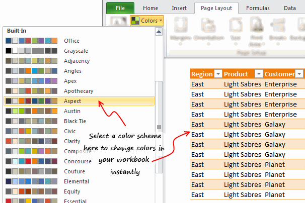
2. Change colors in a snap

So you have made a spreadsheet model or dashboard. And you want to change colors to something fresh. Just go to Page Layout ribbon and choose a color scheme from Colors box on top left. Microsoft has defined some great color schemes. These are well contrasted and look great on your screen. You can also define your own color schemes (to match corporate style). What more, you can even define schemes for fonts or combine both and create a new theme.

3. Use cell styles

Consistency is an important aspect of formatting. By using cell styles, you can ensure that all similar information in your workbook is formatted in the same way. For example, you can color all input cells in orange color, all notes in light gray etc.

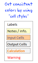
To apply cell styles, just select all the cells you want to have same style and from Home ribbon, select the style you want (from styles area).

Learn how to use cell styles in Excel.

4. Use format painter

Format painter is a beautiful tool part of all Office programs. You can use this to copy formatting from one area to another. See below demo to understand how this works. You can locate format painter in the Home ribbon, top left.

5. Clear formats in a click

Sometimes, you just want to start with a clean slate. May be it is that colleague down the aisle who made an ugly mess of the quarterly budget spreadsheet. (Hey, its a good idea to tell him about Chandoo.org) So where would you start?

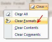
Simple, just select all the cells, and go to Home > Clear > Clear Formats. And you will have only values left, so that you can format everything the way you want.

6. Formatting keyboard shortcuts

Formatting is an everyday activity. We do it while writing an email, making a workbook, preparing a report, putting together a deck of slides or drawing something. Even as I am writing this post, I am formatting it. So knowing a couple of formatting shortcuts can improve your productivity. I use these almost every time I work in Excel.

• CTRL + 1: Opens format dialog for anything you have selected (cells, charts, drawing shapes etc.)


• CTRL + B, I, U: To Bold, Italicize or Underline any given text.


• ALT+Enter: While editing a cell, you can use this to add a new line. If you want a new line as part of formula outcome, use CHAR(10), and make sure you have enabled word-wrap.


• ALT+EST: Used to paste formats. Works like format painter (#4)


• CTRL+T: Applies table formatting to current region of cells


• CTRL+5: To strike thru.


• F4: Repeat last action. For example, you could apply bold formatting to a cell, select another and hit F4 to do the same.

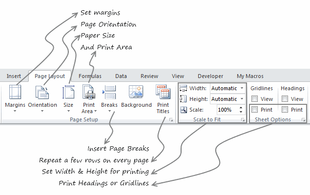
7. Formatting options for print

What looks great on your screen might look messed up, if you do not set correct print options. That is why, make sure that you know how to use these print settings. All of these can be accessed from Page Layout ribbon. For more, you can also use print preview and then “page settings” button.

8. Do not go overboard

Formatting your workbook is much like garnishing your food. No amount of plating & garnishing is going to make your food taste good. I personally spend 80% of time making the spreadsheet and 20% of time formatting it. By learning how to use various formatting features in Excel & relying on productive ideas like tables, cell styles, format painter & keyboard shortcuts, you can save a lot of time. Time you can use to make better, more awesome spreadsheets.

What are your favorite formatting tips?

Formatting (or making something look good) helps you get great first impression. I am always looking for ways to improve my formatting skills. While a great deal of formatting skill is art (and personal taste), there are several ground rules to follow as well. Applying ideas like consistency, alignment, simplicity and vibrancy goes a long way.

What formatting tips & ideas you follow? Please share them with us using comments.

Learn how to make better spreadsheets

• 10 tips to make spreadsheets that your boss will love


• 5 Ways to use conditional formatting to make awesome spreadsheets


• 12 Rules for making better spreadsheets


• More tips on formatting, conditional formatting, custom cell formatting & chart formatting

Join Excel School & Make awesome Excel sheets

In my Excel School program, we focus not just on teaching Excel, but also teaching you how to make awesome Excel workbooks. You can see how I format my data, charts, dashboards & reports and learn hundreds of tips on formatting.

Even the lesson workbooks are beautifully formatted & packed with fresh ideas for you to try.

Consider joining our Excel School program, because you want to be awesome in Excel.

Copy Data to Another Worksheet with Advanced Filter

From Excel Semi-Pro

Copy Data to Another Worksheet with Advanced Filter:

Dear Microsoft, please fix the Advanced Filter in Excel. Copying filtered data to another worksheet should be simple but it’s not. Fixing this would help out many of your beginning and intermediate users and some of us old dogs who seemingly haven’t learned the trick.

The Problem with Advanced Filter in Excel

I was reading a post on the Contextures Blog, which indicated that you could use the Advanced Filter feature in Excel to copy filtered data to another worksheet. This feature has the potential to shorten some of my VBA code that essentially does the same thing. I mean, using Excel to do the work is simpler and usually faster than writing the code yourself.

So I created a simple worksheet with dummy data and tried out the Advanced Filter feature. In the picture below my List Range and Criteria Range are on Sheet1 and I’m just about to Copy to another location: Sheet2.

However, when I click the OK button the following message pops up.

The Trick to Copy Filtered Data to Another Worksheet

My problem was that I didn’t know the secret. You have to initiate the Advanced Filter from the worksheet you are going to copy to. Duh, stupid me. So here’s how I defeated my nemesis, the Advanced Filter.

1. Activate sheet 2 (where the data goes)


2. Choose Data > Advanced Filter


3. Select the List Range on sheet 1


4. Select the Criteria range on sheet 1


5. Select the radio button: Copy to another location


6. Select the Copy to range on sheet 2


7. Click OK

Here is the resulting data copied to Sheet 2.

There is a short video from Debra Dalgleish on how this is done. I’m too frustrated with Microsoft to pull off a video without disdain in my voice.

The problem I’m having is that this “work around” has been required for quite some time, with no updating of the Excel software code by Microsoft. (The video link above is for Excel 2003.) And yet in the latest two versions of Excel, 2010 and 2011, we still have to do something, that seems to me to be, completely counter-intuitive and un-productive.

Advanced Filter with VBA

I turned on the macro recorder to document the code required to execute, what I’m calling a “work around.” I then copied the first macro, modified the code, and ran it again from sheet 1 and it worked just fine.

The first macro: CopyToOtherSheet does two things. 1) Selects Sheet 2 because that is what Microsoft requires, then 2) uses the AdvancedFilter method of the Range property to FilterCopy the CriteriaRange to the CopyToRange, with no Unique records.

The second macro: FilterCopyToOtherSheets only does one thing. It does what Microsoft should have done long ago, and that’s to copy the filtered range (sheet 1) to the copy range (sheet 2) while your on sheet 1.

The only code I changed (highlighted in red) was to eliminate the selection of Sheet 2, and add Sheets(“Sheet2″). to the CopyToRange. You can run this macro from Sheet 1 and the Advanced Filter will copy the filtered data to Sheet 2 with no problems.

Of course with static ranges this is a very limited macro, but my point here is that the code change should be minimal and if Microsoft can spend several billion dollars to get Windows 7 into Nokia phones, this shouldn’t cost to much to fix.

Okay, I’m done ranting.

Helpful Links

Excel’s Advanced Filter Help Online

Excel AutoFilter or Advanced Filter?

From Contexture.com

Excel AutoFilter or Advanced Filter?:

Do you ever use the Excel Advanced Filter feature? Or is all your filtering done with an AutoFilter?

AutoFilter Benefits

For ease of use, it’s hard to beat the Excel AutoFilter feature. Just click the Filter command on the Excel Ribbon’s Data tab, and the filter is ready to go.

You can click the drop down arrows in the column headings, and use the check boxes to select the items you want in the filter. Or, use the Text, Date or Number Filters commands, for variations on the filters.

Another quick way to filter is to right-click on a cell in the list, then click Filter, and click Filter by Selected Cell’s Value.

Advanced Filter Benefits

The Excel Advanced Filter isn’t as easy to use (I guess that’s why they call it Advanced ), but it does have some benefits that make it worth the effort.

After you click the Advanced command on the Excel Ribbon’s Data tab, the Advanced Filter dialog box opens. Fill in the details, and then click the OK button to filter the data.

Filter Data to Anther Sheet

The main reason that I use an Advanced Filter, especially when programming in Excel, is that it’s a quick and efficient way to copy specific data to a different worksheet.

In the screen shot above, the option is selected to copy the filtered data to another location. You can use that option to quickly create a report for each department, or salesperson, and email the results.

Create a List of Unique Items

Excel 2007 introduced the Remove Duplicates feature, but I still use an Advanced Filter to create lists of unique items. The Remove Duplicates feature strips the duplicates out of the list that is selected, so you have to remember to work on a copy of the list, if you want to keep the original list intact.

With an Advanced Filter, no items are removed from the list, so you don’t risk losing any of your original data.

Complex Filters

With an Advanced Filter, you can create a criteria range on the worksheet, and see at a glance what the filter settings are. You can also create complex filters with AND/OR settings that go beyond what an AutoFilter can do.

For example, with an AutoFilter, you can select two specific customers, and two products for those selected customers.

With an Advanced Filter, you can create OR conditions between columns, such as Customer A OR Product B — you can’t do that in an AutoFilter!

_________

Display Contact Group Member Count

From Code for Excel and Outlook

Display Contact Group Member Count:

Sorry for the lack of posts lately. I've been working on the next version of Random Data Generator, and my home network connection wasn't working for the past few days.

In Display the Total Number of Members in a Contact Group there is a method for displaying the number of members of a contact group (aka distribution list).

There is an easier way, using VBA:

Sub GetDistListCount()

Dim dl As Outlook.DistListItem

Set dl = ActiveExplorer.Selection.item(1)

MsgBox "There are " & dl.MemberCount & " member(s) in this contact group."

End Sub

Just go to your Contacts folder, select a distribution list item and run this code. There is no error handling here, just a simple procedure to display the number of members of the group.

Related Articles:

• June 23, 2011 -- Manage your email overload
• March 7, 2011 -- Get Word Count in VBA
• January 31, 2011 -- Add photos to Contacts in bulk using VBA in Outlook

Display Contact Group Member Count is Copyright © JP Software Technologies. All Rights Reserved.

Finding the 2nd, 3rd, 4th … MATCH()

From Daily Does of Excel

Finding the 2nd, 3rd, 4th … MATCH():

Excel’s MATCH() function will return the relative location of the first occurrence that satisfies the match criterion (the lookup_value) within the specified array (the lookup_array). Most often, this is what you want. For instance, if you have duplicate entries, returning the first match is no different than returning the last match. However, if you have unique entries with the duplicated criterion, how do you return all the unique values?

For example, you have a list of the 122 major professional sports teams (32 NFL, and 30 MLB, NBA, and NHL) sorted alphabetically in Column D. In Column E you have code that returns the length of the team name, i.e. =LEN(D1). Your data might look like this:

	D	E
1	Anaheim Ducks	13
2	Arizona Cardinals	17
3	Arizona Diamondbacks	20
4	Atlanta Braves	14
5	Atlanta Falcons	15
6	Atlanta Hawks	13
7	Baltimore Orioles	17
8	Baltimore Ravens	16
9	Boston Bruins	13
10	Boston Celtics	14

For no good reason we want to create a descending sort on name length. You can do it from the Sort selection, but we also want to keep the alpha-sort. In F1 you put =LARGE($E$1:$E$122,ROW()) and fill down. The ROW() function will cause the return of the first largest, then the second largest etc. Then you want to know how far down Column E those descending numbers fall, so that you can Index the name list that amount. In G1 put the code =MATCH(F1,$E$1:$E$122,0) and fill down. You’ll see from the data that the longest name is 29 letters, and it’s in ROW(52).

	D	E	F	G
1	Anaheim Ducks	13	29	52
2	Arizona Cardinals	17	22	30
3	Arizona Diamondbacks	20	22	30
4	Atlanta Braves	14	22	30
5	Atlanta Falcons	15	21	42
6	Atlanta Hawks	13	21	42
7	Baltimore Orioles	17	21	42
8	Baltimore Ravens	16	20	3
9	Boston Bruins	13	20	3
10	Boston Celtics	14	20	3

You can begin to see the problem: There are three teams with a 22-letter name, three with a 21-letter name, and at least 3 (in fact 13) with a 20-letter name. If in H1 we put =INDEX(D:D,G1) and filldown, we get:

	D	E	F	G	H
1	Anaheim Ducks	13	29	52	Los Angeles Angels of Anaheim
2	Arizona Cardinals	17	22	30	Columbus Blue Jackets
3	Arizona Diamondbacks	20	22	30	Columbus Blue Jackets
4	Atlanta Braves	14	22	30	Columbus Blue Jackets
5	Atlanta Falcons	15	21	42	Golden State Warriors
6	Atlanta Hawks	13	21	42	Golden State Warriors
7	Baltimore Orioles	17	21	42	Golden State Warriors
8	Baltimore Ravens	16	20	3	Arizona Diamondbacks
9	Boston Bruins	13	20	3	Arizona Diamondbacks
10	Boston Celtics	14	20	3	Arizona Diamondbacks

This is exactly what we wanted to avoid. So, using Col(H) now as a helper column, in H1 put =G1. In H2 put

• =IF(G2<>G1,G2,H1+MATCH(F2,INDIRECT(“E”&(H1+1)&”:E122″),0))

and fill down. If the value did not repeat, just copy it over; and if it didn’t, we’re making a “sliding range” that starts one row after the start of a repeated pair, ends at the end of the data, and “slides” down Column E. The sliding range is made by the INDIRECT() function. It builds the range one row down (H1+1) from the first of a repeating match. We add H1 to that result, and we have our index down Column D. This may be better seen in H3, adjacent to G3, where the first repeat starts.

• =IF(G3<>G2,G3,H2+MATCH(F3,INDIRECT(“E”&(H2+1)&”:E122″),0))

The IF() is false. We are looking for the relative location of the lookup_value (22) in a new lookup_range (E31:E122). It’s 33 rows in. We add the original 30 to that, and the index is now 63. A similar thing happens in H4. H5 is G5 copied over. In Column I, I1 =INDEX(D:D,H1), filled down. The resulting table:

	D	E	F	G	H	I
1	Anaheim Ducks	13	29	52	52	Los Angeles Angels of Anaheim
2	Arizona Cardinals	17	22	30	30	Columbus Blue Jackets
3	Arizona Diamondbacks	20	22	30	63	Minnesota Timberwolves
4	Atlanta Braves	14	22	30	95	Portland Trail Blazers
5	Atlanta Falcons	15	21	42	42	Golden State Warriors
6	Atlanta Hawks	13	21	42	83	Oklahoma City Thunder
7	Baltimore Orioles	17	21	42	89	Philadelphia Phillies
8	Baltimore Ravens	16	20	3	3	Arizona Diamondbacks
9	Boston Bruins	13	20	3	49	Jacksonville Jaguars
10	Boston Celtics	14	20	3	53	Los Angeles Clippers

The names are now sorted by length, by alphabet. INDIRECT() is volatile, so there is a penalty for this. For extra credit, and no peeking, what’s the shortest name?

…mrt

©¿©¬

Is it Standard Time yet?

From: Daily Does of Excel

Is it Standard Time yet?:

Part of my part-time job schedules world-wide PC-chat conferences weekly, and I announce the time referenced to the East Coast. As daylight savings time is about to end, I wanted an algorithm that knew whether standard time or daylight savings time was in effect.

As I’m not worried about the 2:00AM change over, I can do it based on the date. Since 2007, if the month is December through February, standard time is in effect. If the month is April through October, daylight savings time is in effect. Daylight savings time starts the second Sunday in March, and ends the first Sunday in November.

So, by counting Sundays in March and November, I can toggle the time zone. This is what I came up with.

Function TZ(SomeDay As String) As String

Dim TestDay As Long, TestMonth As Long, TestYear As Long

Dim IsDST As Boolean

Dim i As Long, SundayCount As Long

TestDay = VBA.Day(SomeDay)

TestMonth = VBA.Month(SomeDay)

TestYear = VBA.Year(SomeDay)

IsDST = False ‘months 1, 2, 12

Select Case TestMonth

Case 3

For i = 1 To TestDay

If VBA.Weekday(VBA.DateSerial(TestYear, 3, i)) = 1 Then SundayCount = SundayCount + 1

If SundayCount = 2 Then

IsDST = True

Exit For

End If

Next i

Case 4, 5, 6, 7, 8, 9, 10

IsDST = True

Case 11

For i = 1 To TestDay

If VBA.Weekday(VBA.DateSerial(TestYear, 11, i)) = 1 Then SundayCount = SundayCount + 1

If SundayCount = 1 Then Exit For

Next i

If SundayCount = 0 Then IsDST = True

End Select

If IsDST Then TZ = “EDT” Else TZ = “EST”

End Function

The default WEEKDAY() function returns 1 for Sunday, so if there are 2 Sundays in March including the day in question, turn IsDST to TRUE, and stop the loop. Conversely, if there is 1 Sunday in November including the day in question, leave IsDST as FALSE, and stop the loop.

I use the VBA. leader to ensure this function works on a Mac. Needless to say, it also works in MSWord.

…mrt
©¿©¬

Posting Code to this Blog

From : Daily Does of Excel

Posting Code to this Blog:

For years I’ve been typing <code> tags and pasting code between them. But no more! I wrote a small utility that puts the code tags around my code and pops into the clipboard. Think of the seconds that I’ll save.

There are three situations that I wanted to cover with this code; no selection, multiple procedure selection, and intra-procedure selection. If there’s no selection, I want the whole procedure that contains the cursor. If the selection spans more than one procedure, I want the entirety of all the procedures that are touched by the selection. If the selection is within one procedure, I want what’s selected.

This code uses the Microsoft Visual Basic Extensibility library.

To get this	Select this

Sub CreateCodeTags()



Dim cp As CodePane, cm As CodeModule

Dim lStartLine As Long, lEndLine As Long

Dim lStartCol As Long, lEndCol As Long

Dim sStartProc As String, sEndProc As String

Dim lStartType As Long, lEndType As Long

Dim sOutput As String

Dim doClip As DataObject



Set cp = Application.VBE.ActiveCodePane

Set cm = cp.CodeModule



cp.GetSelection lStartLine, lStartCol, lEndLine, lEndCol



sStartProc = cm.ProcOfLine(lStartLine, lStartType)

sEndProc = cm.ProcOfLine(lEndLine, lEndType)



‘Single cursor = get whole procedure

If lStartLine = lEndLine And lStartCol = lEndCol Then

sOutput = cm.Lines(cm.ProcStartLine(sStartProc, lStartType) + 1, cm.ProcCountLines(sStartProc, lStartType) – 1)

‘Spans more than one procedure = get all procedures in selection

ElseIf sStartProc <> sEndProc Then

lStartLine = cm.ProcStartLine(sStartProc, lStartType) + 1

lEndLine = cm.ProcStartLine(sEndProc, lEndType) + cm.ProcCountLines(sEndProc, lEndType)

sOutput = cm.Lines(lStartLine, lEndLine – lStartLine)



‘Same line = get selected text

ElseIf lStartLine = lEndLine Then

sOutput = Mid$(cm.Lines(lStartLine, 1), lStartCol, lEndCol – lStartCol)



‘Multiple lines = get selected text

Else

sOutput = Mid$(cm.Lines(lStartLine, 1), lStartCol, Len(cm.Lines(lStartLine, 1)))

If lEndLine – lStartLine > 1 Then

sOutput = sOutput & vbNewLine & cm.Lines(lStartLine + 1, (lEndLine) – (lStartLine + 1))

End If

sOutput = sOutput & vbNewLine & Left$(cm.Lines(lEndLine, 1), lEndCol – 1)

End If



If Right$(sOutput, Len(vbNewLine)) = vbNewLine Then

sOutput = Left$(sOutput, Len(sOutput) – Len(vbNewLine))

End If



sOutput = “< code lang=”“vb”“>” & sOutput & “< /code>”



Set doClip = New DataObject



doClip.SetText sOutput

doClip.PutInClipboard



End Sub

In the last line that begins with

<span class="vb">sOutput =</span>

I had to add some extraneous spaces to be able to post code that contains code tags, but they’re not really there in the code.

Other than that I’m merely doing string manipulation with my starting and ending lines and columns.

I think I need to add the

<span class="text">inline = "true"</span>

argument when I’m on a single line. I think I’ll use and see how often I’m adding it.

Display Contact Group Member Count

From : Code For Excel And Outlook - Learn VBA »

Display Contact Group Member Count:

Sorry for the lack of posts lately. I've been working on the next version of Random Data Generator, and my home network connection wasn't working for the past few days.

In Display the Total Number of Members in a Contact Group there is a method for displaying the number of members of a contact group (aka distribution list).

There is an easier way, using VBA:

Sub GetDistListCount()

Dim dl As Outlook.DistListItem

Set dl = ActiveExplorer.Selection.item(1)

MsgBox "There are " & dl.MemberCount & " member(s) in this contact group."

End Sub

Just go to your Contacts folder, select a distribution list item and run this code. There is no error handling here, just a simple procedure to display the number of members of the group.

Related Articles:

• June 23, 2011 -- Manage your email overload
• March 7, 2011 -- Get Word Count in VBA
• January 31, 2011 -- Add photos to Contacts in bulk using VBA in Outlook

Display Contact Group Member Count is Copyright © Code For Excel And Outlook - Learn VBA. All Rights Reserved.